¶ Description
Aggregate (or Group By) rows.
¶ Parameters
¶ Standard tab
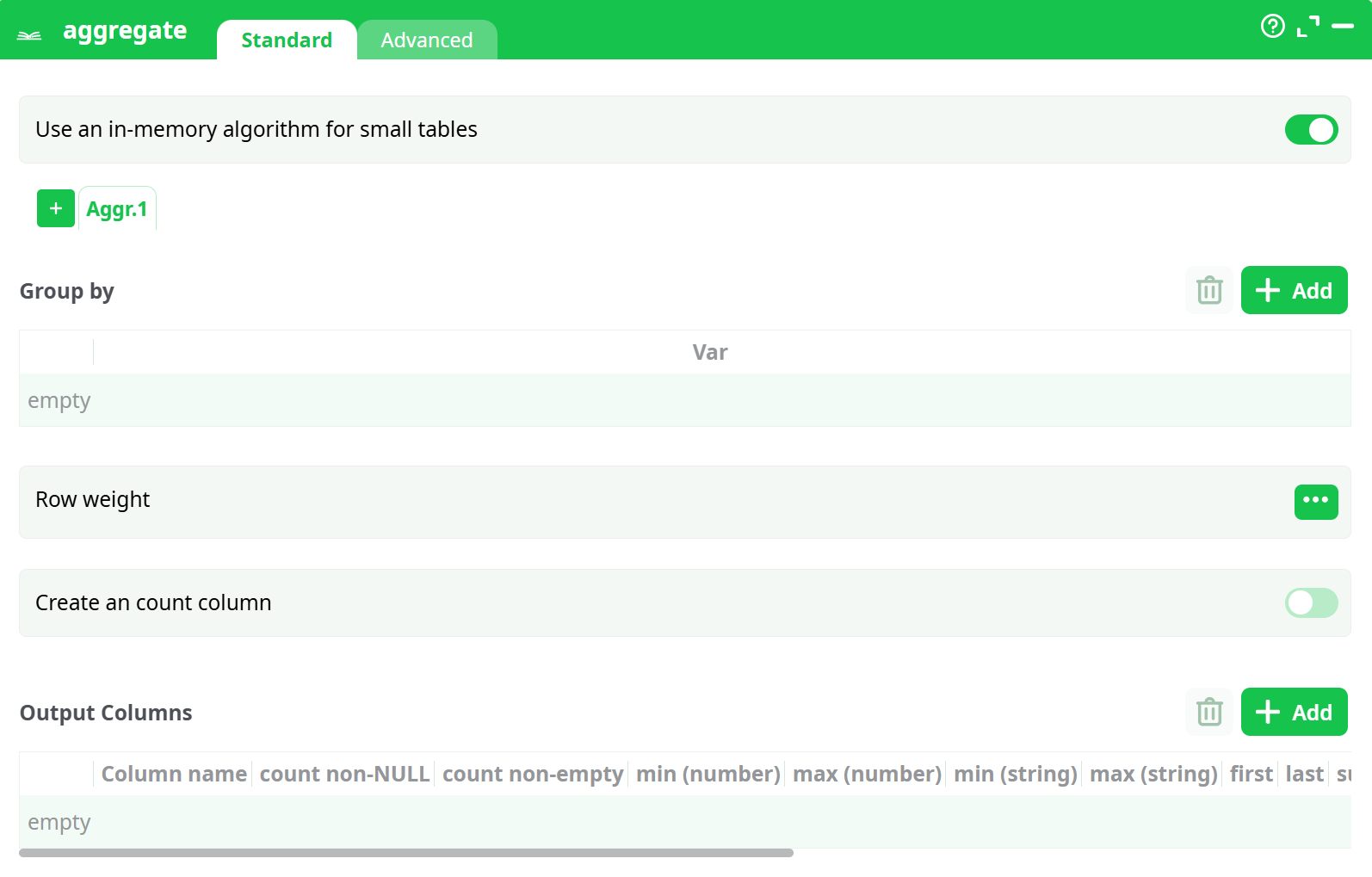
Parameters:
- Group by
- Use an in-memory algorithm for small tables
- Row weight
- Create an count column
- Output Columns
¶ Advanced tab
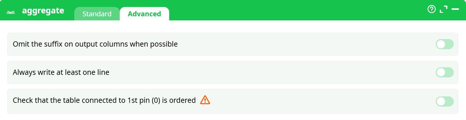
Parameters:
- Omit sufix on output column if possible
- Always write one line at least
- Check table connected to first pin is ordered
¶ About
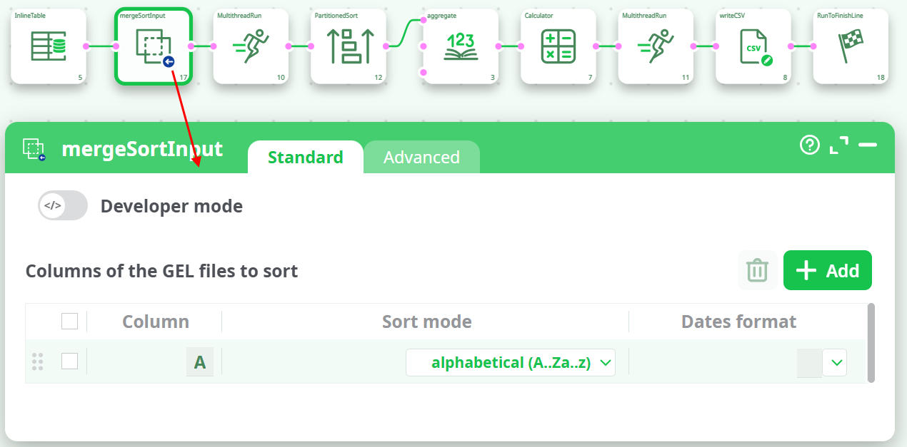
You can click on the header of the “output column table” to check all the checkboxes of the column. If you don’t provide any “group by” variables, the whole input table will be used to compute only one output row. For example, these settings:
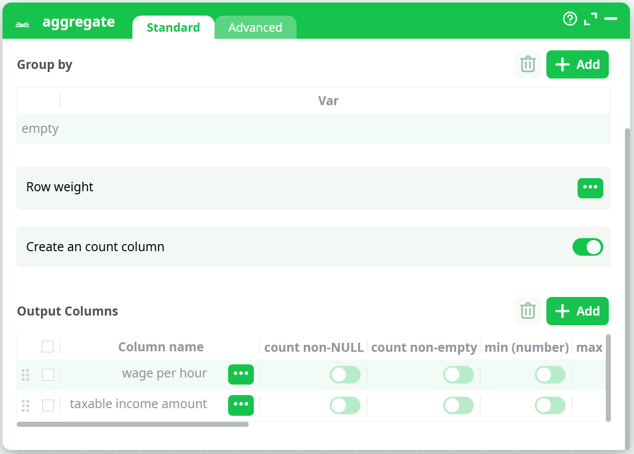
… will generate a one-row output table with the 2 columns “wage per hour_mean” and “taxable income amount_mean”.
You can give several “Group by” variables, there will be as many output rows as there are of modality-combinations into your data. For example, if your “Goup-By-variables” are: Wealth (Poor, Rich), Age (Young, Middle, Old), Sex (Woman, Man), then you will have as output these 12 rows:
| Idx | Wealth | Age | Sex |
|---|---|---|---|
| 1 | Poor | Young | Woman |
| 2 | Poor | Young | Woman |
| 3 | Poor | Middle | Woman |
| 4 | Poor | Middle | Woman |
| 5 | Poor | Old | Woman |
| 6 | Poor | Old | Woman |
| 7 | Rich | Young | Man |
| 8 | Rich | Young | Man |
| 9 | Rich | Middle | Man |
| 10 | Rich | Middle | Man |
| 11 | Rich | Old | Man |
| 12 | Rich | Old | Man |
Note that the combination (Rich,Young,Man) is very un-likely, so it might not appear as output in the result table.
There are two operating modes for this action:
¶ In-Memory Mode.
In this mode, ETL builds all the output table(s) in memory (and there can be multiple output tables).
ETL reads the input table row by row. Each time a new combination (technically called a "t-uple") is found in the input table, ETL extends the in-memory result table by adding a new row to store the aggregations for that specific combination. If a known combination is found, ETL simply updates the existing aggregation to include the new input row.
In this mode, ETL reads the entire input table before producing any output rows.
This mode is very memory-intensive because all output tables must fit into RAM. If your output tables do not fit into memory (e.g., larger than 2GB on a 32-bit system), ETL may fail to compute the aggregation or become extremely slow due to memory swapping.
Therefore, if your output tables are very large, you should use the Out-of-Memory Mode.
When using the “in-memory” mode, the Aggregate action cannot be included inside a “N-Way Multithread Section”.
¶ Out-of-Memory Mode.
This mode allows ETL to compute any aggregation, regardless of the size of the (single) output table.
To use this mode, your input table must be sorted by the Group By variables. This requirement can be inconvenient, as sorting is typically a very slow operation and should be avoided when possible. Therefore, if your output tables are small, it's better to use In-Memory Mode—unless the input table is already sorted "for free."
ETL reads the input table row by row. Thanks to the sorting, all rows with the same combination (i.e., the same values for the Group By variables—technically referred to as the same "t-uple") are contiguous. When ETL encounters the same combination again, it simply updates the aggregation to include the new input row. If the combination changes, ETL immediately generates a new output row with the aggregation values for the t-uple that just ended.
In this mode, ETL produces output rows as it reads the input table.
This mode consumes minimal memory, in contrast to In-Memory Mode.
When using the “out-of-memory” mode, the Aggregate Action can be included inside a “N-Way Multithread Section”, provided that the input table is still correctly sorted on the “Group by” variables.
¶ Using the “in-memory mode” to compute several aggregations simultaneously
When using the In-Memory Mode of the Aggregate action, you can compute multiple aggregations (i.e., output tables) simultaneously. For example, the following two ETL pipelines are functionally equivalent, but the second one is at least twice as fast as the first:
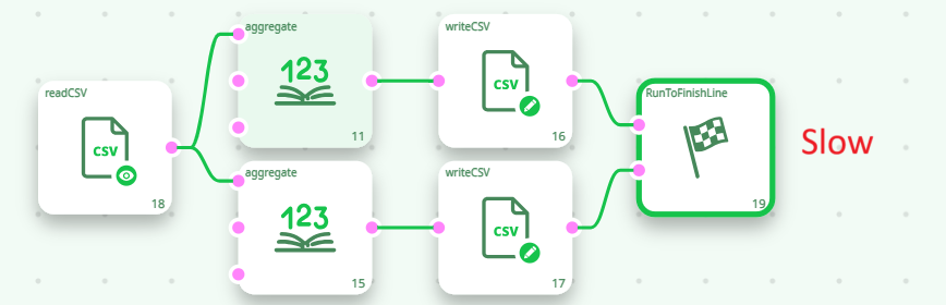
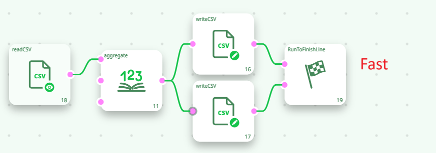
Inside the second pipeline here above, we used the fact that the ETL Aggregate action is able to compute several aggregation tables “in parallel”, requiring only one pass over the database to compute all the aggregation tables. This is a unique functionality of ETL. Thanks to this functionality, the running-time of an ETL-transformation-pipeline containing several aggregations is usually divided by 2 or 3 (or even 4) compared to a standard implementation based on ELT techniques and simple SQL scripts. ETL delivers you high-performance & ultra-fast computations!
¶ Optimizing the sort before the “out-of-memory” Aggregate
Let’s assume that we have:
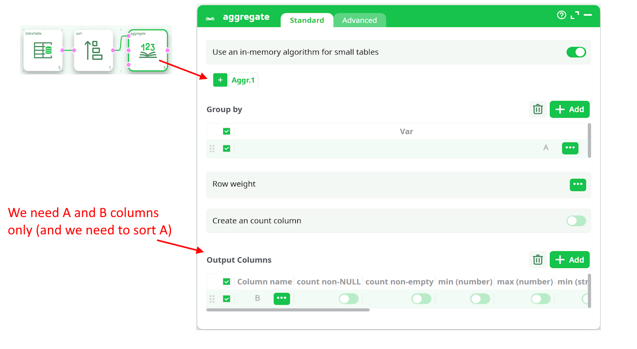
In such situation, we can do the following:
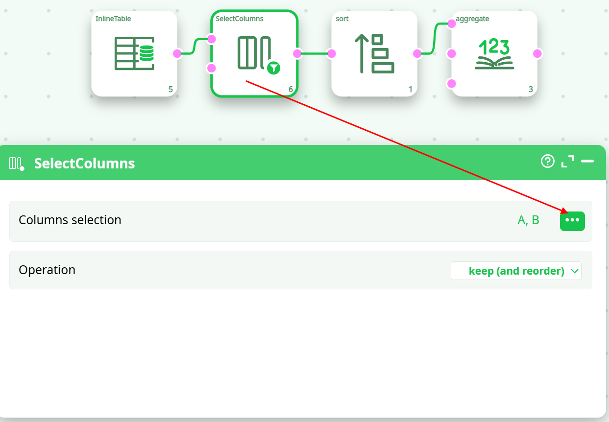
To compute the above aggregation, we only need to sort a table containing only the A and B columns (not the entire table with all columns). Therefore, it's useful to place a ColumnFilter action before the Sort action. To achieve the highest computation speed, you should always minimize the volume of data being sorted.
¶ Using the “out-of-memory mode” inside a N-Way Multithreaded Section
Let’s assume that we want to multithread/parallelize this simple ETL Transformation Pipeline:
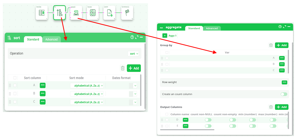
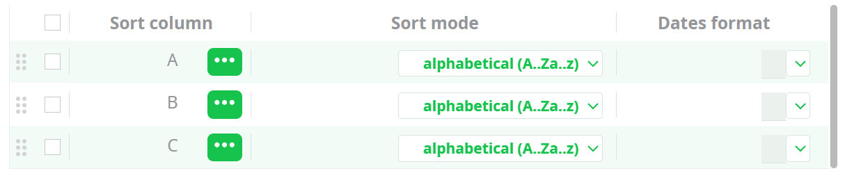
When the Aggregate Action starts, it looks at the meta-data of the input table to check if it’s properly sorted on the columns A, B & C. …And since that’s the case (because of the Sort Action running in “Check sort with error” mode), it can proceed computing the aggregations.
The above pipeline is equivalent to the SQL command:
SELECT sum(D) as D_sum, sum(E) as E_sum, mean(D) as D_mean, mean(E) as E_mean, FROM table GROUP BY A,B,C
…followed by some small computation based on A, B, C, D, D_sum, E_sum, D_mean, E_mean.
Let’s now include the Aggregate action, inside a N-Way Multithread Section:

By default, the above pipeline won’t run because the meta-data of the input table of the Aggregate Action says that the input table is not sorted (by default, any sort-meta-data is lost at the start of the N-Way Multithread Section). To “keep” the sort-meta-data inside the interior of the N-Way Multithread section, we must set the partitioning parameter of the second Multithread action to “A”:
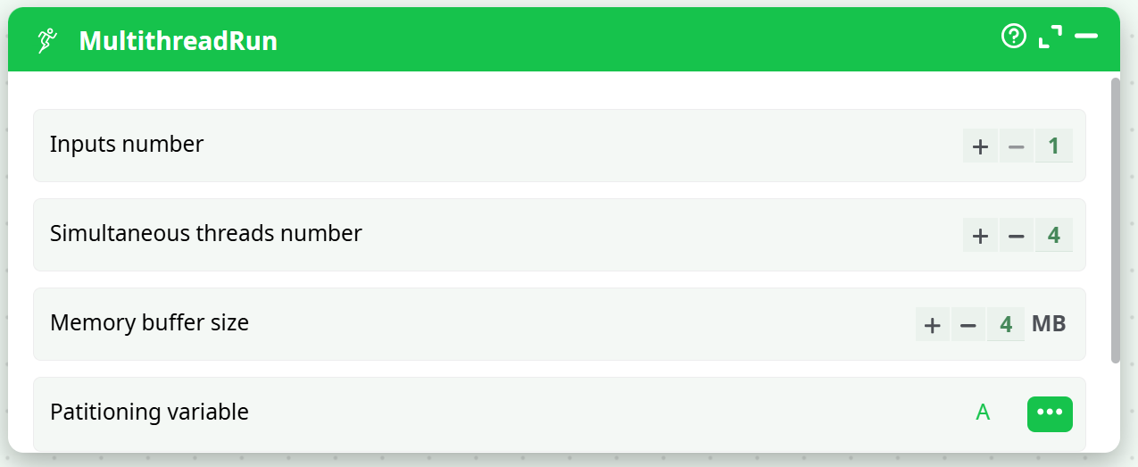
This is a special case: When the partitioning parameter is equal to the most significant column of the sort-meta-data, then the sort meta-data is kept inside the interior of the N-Way Multithread section. (So that the Aggregate action works, once again, properly)
Let’s now assume that the text file that is used as source data for the ETL pipeline is sorted on the column A only (and not on the columns A, B & C, as previously). We’ll thus have:
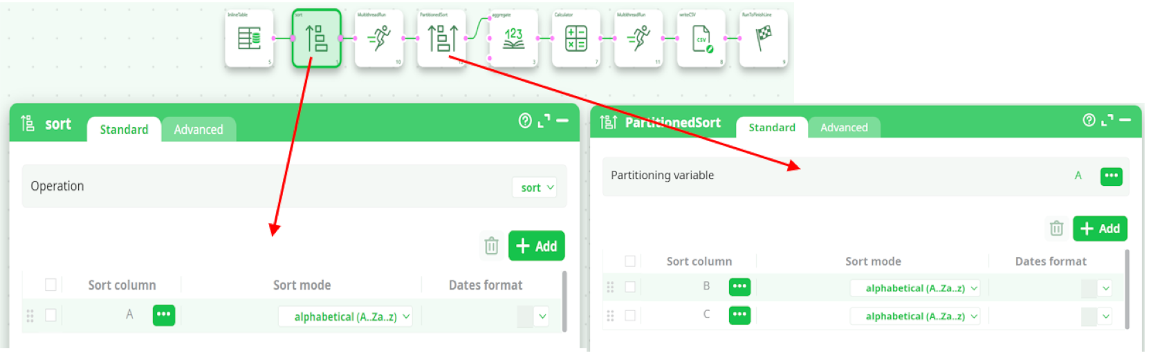
In the general case, the output table of the PartitionedSort action is not sorted (i.e. it does not contain any sort-meta-data at all). In the above example, we are in a special case: The partitioning variable of the PartitionedSort action is equal to the most-significant sort-variable of the input table. In this special case, the sort-meta-data of the output table is not empty. In the above example, the sort-meta-data is automatically set to:
(So that the Aggregate Action works, once again, properly!)
The above ETL pipeline is very efficient because:
- It computes aggregations using many CPUs (because the Aggregate action is inside a N-Way Multithread section).
- The aggregations are computed using the “out-of-memory” mode, meaning that we can handle output tables of unlimited size.
- When using the “out-of-memory” mode to compute aggregation, the input table must be sorted on all the “group by” variables. In the above example, the input table was only partially sorted on one of the “group by” variable (i.e. it was sorted only on the column A, but not on the columns B and C). Although the source table was not properly sorted, we were nevertheless able to compute the aggregations, thanks to the Partitioned Sort Action that “extended” the sort-meta-data (to include the columns B and C) so that the Aggregate action still works properly.
- We were able to run on many CPUs the PartitionedSort action (because it’s inside a N-Way Multithread section). Usually, sorting is a very slow operation and thus it’s very nice to be able to easily use many CPU’s to sort the data because it reduces considerably the computation time.
- It’s using a very small amount of RAM memory (there are no Sort Action and the Aggregate Action are running in “out-of-memory” mode).
¶ Avoiding a costly “sort”
In the above example, we assumed that the text file that is used as source data for the ETL pipeline is sorted on the column A. If that’s not the case, we can use the following procedure:
- Read the source text file and write it back inside many different .gel files using the “split variable” option of the writeGel Action. For example, this ETL pipeline splits the data in different .gel file, one file per each different day:
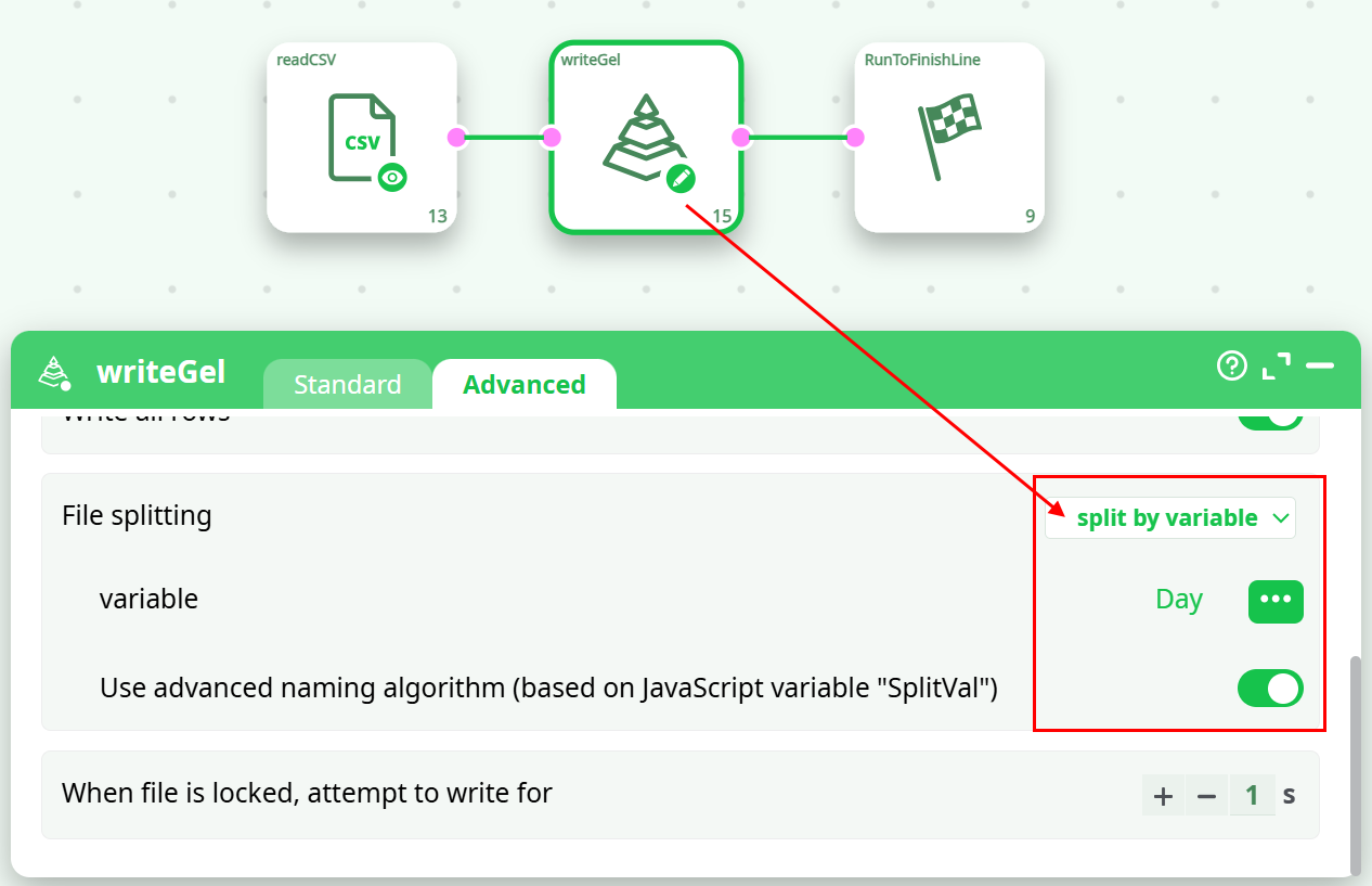
-
Sort all the different .gel files that were produced at the precedent step. This sort can easily be run in parallel (one CPU for each different day/file).
I suggest you to use the “ProcessRunner” JavaScript class to run on parallel on several CPUs an ETL pipeline that sorts (using a simple Sort action) one particular day that is specified as command-line parameter to the pipeline (i.e. as “Pipeline Global Parameter”).
Although we are using the simple Sort action, we still get high speed because:- We are able to run the sort on many CPUs (one CPU per each different day/file).
- The volume of data to sort is limited (it’s only one day) and it can happen that the Sort Action is able to perform the sort entirely in RAM-memory (without using any tape files). When this happens, the sort is a lot faster.
- If the data arrives on a daily basis, we can avoid re-computing all the sorts for all the previous days (by keeping on the hard drive the sorted .gel files that were previously computed) and we only sort the “last” file/day that we just received. This leads to a somewhat “incremental” sorting algorithm that only needs to sort a very small quantity of data before being able to compute very efficiently large aggregates.
-
Use the MergeSortInput action (or the MergeSort action) to obtain, from the different “locally sorted” .gel files, one “globally sorted” table. We’ll have:
This last data-transformation-pipeline is even more efficient than the previous one because:
- it starts from a set of “locally sorted” file (i.e. we used the term “locally” because we sorted “locally” each day/file on the column A and we managed to avoid sorting “globally” ALL the data from ALL the days).
- Each day/file is only “partially” sorted (i.e. each day is sorted on the column A only).
- It allows you to use an “incremental” sorting algorithm that reduces the computing time by several orders of magnitude. We used the term “incremental” because we only need to sort the small quantity of new days of data that we just received (and not all the days).
- It manages to keep the 5 advantages that were explained for the previous ETL pipeline:
- It computes aggregations using many CPUs (still reducing computing time).
- You can have output tables of unlimited size.
- It’s not using any Sort actions (that are slow and memory hungry).
- The little amount of sorting is performed on many CPUs (still reducing computing time).
- It’s using a very small amount of RAM memory.
¶ Dynamic Aggregation
It can happen on some occasion that you don’t know “in advance” the precise nature of the aggregation that you want to compute: i.e. you need to run some computation to now exactly which aggregations to compute. In such situation, you should use the second and third input pin (pin 1 and 2) from the Aggregate action. More precisely,
- The second table contains the “group by” information. It only has one column that contains the names of all the “group by” columns.
- The third table contains the “output column” information. It only has two columns:
- The first column is the name of the variable to process/aggregate.
- The second column contains a string that describes the aggregate to compute. The accepted values are (case insensitive):
- IMin (number minimum)
- IMax (number maximum)
- SMin (string minimum)
- SMax (string maximum)
- First
- Last
- Sum
- Mean
- StdDev
- CountDistinct
- CountNonEmpty
- CountNonNull
- MostCommonModality
- CountMostCommonModality