¶ Description
Linear regression on variables.
¶ Parameters
¶ Parameters tab
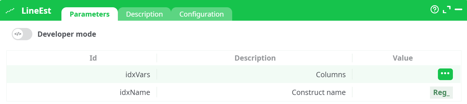
Parameters:
- Columns
- Construct name
¶ Description tab
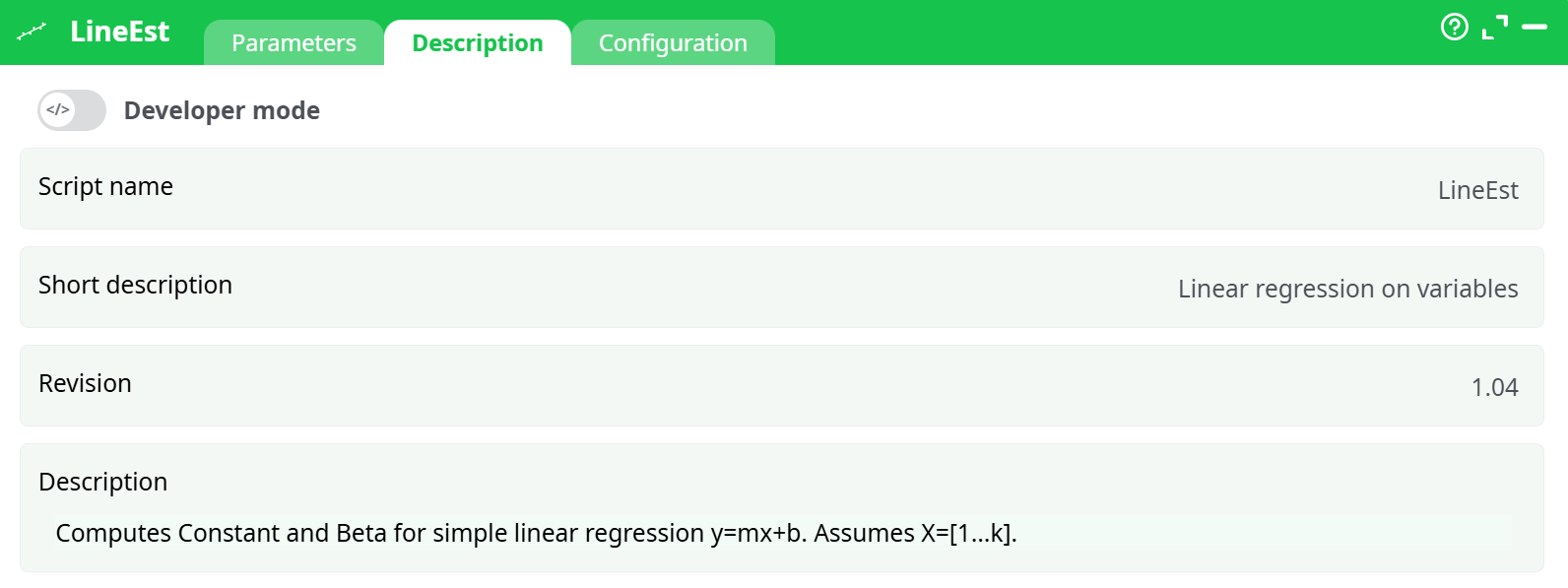
Parameters:
- Script name
- Short description
- Revision
- Description
¶ Configuration tab
See dedicated page for more information.
¶ About
The LineEst action button computes a simple linear regression for each row in the dataset. It assumes that each column represents values at equal time intervals (e.g., monthly purchases), and fits a line y = mx + b (where m = Beta, b = Constant) across these columns.
This transformation is particularly useful when working with time series data in wide format—especially for detecting trends in customer behavior or sales over time. For example, you may have monthly data points across several columns, and you'd like to determine the upward or downward trend for each customer individually.
¶ Use Cases
- Customer Behavior Analysis: Calculate trends in customer activity (purchases, visits, etc.) over the past 3, 6, 12, or 24 months.
- Segmentation Input: Use computed Beta (slope) and Constant (intercept) values as simplified inputs for clustering or predictive modeling.
- Trend Identification: Spot customers with rising or falling activity, and trigger marketing or risk management workflows accordingly.
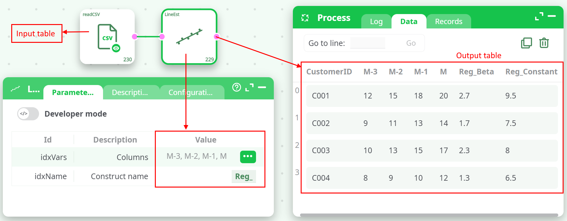
¶ Input Example
The input table should contain one identifier column (e.g., CustomerID) followed by time-series columns, where each column represents a snapshot in time (e.g., M-3, M-2, M-1, M):
| CustomerID | M-3 | M-2 | M-1 | M |
|---|---|---|---|---|
| C001 | 12 | 15 | 18 | 20 |
| C002 | 9 | 11 | 13 | 14 |
| C003 | 10 | 13 | 15 | 17 |
| C004 | 8 | 9 | 10 | 12 |
Note: The order of the time columns matters. They must be chronologically ordered from oldest (left) to newest (right).
¶ Output Example
The output table includes the original columns plus two new ones:
- Reg_Beta – the slope of the regression line.
- Reg_Constant – the y-intercept of the regression line.
¶ Parameters
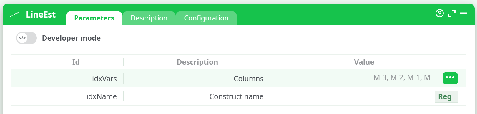
The generated output columns will be named: Reg_Beta and Reg_Constant.
¶ Internal Logic
The LineEst action estimates a simple linear regression model of the form:
Y = mX + b
Where:
Xis a sequence of time points (1, 2, ..., k),Yis the row's values across time-series columns,m(Beta) represents the trend (positive, negative, or flat),b(Constant) is the value of the regression line when X = 0.
The regression is computed per row, meaning each row is treated independently, and each gets its own Beta and Constant.
Notes
- Only numeric columns should be selected for regression.
- All selected columns must contain non-null, numeric values for each row. Missing or invalid data may result in null output.
- Works best with time-aligned data (equal interval between columns).
¶ Summary
The LineEst action simplifies time-series data into trend components (slope and intercept), making further analysis more efficient and interpretable. It is an essential tool for behavioral analytics, forecasting, and feature engineering for machine learning models.