¶ Description
Create a JSON file that contains a table coming from the ETL transformation pipeline.
¶ Parameters
¶ Standard Tab
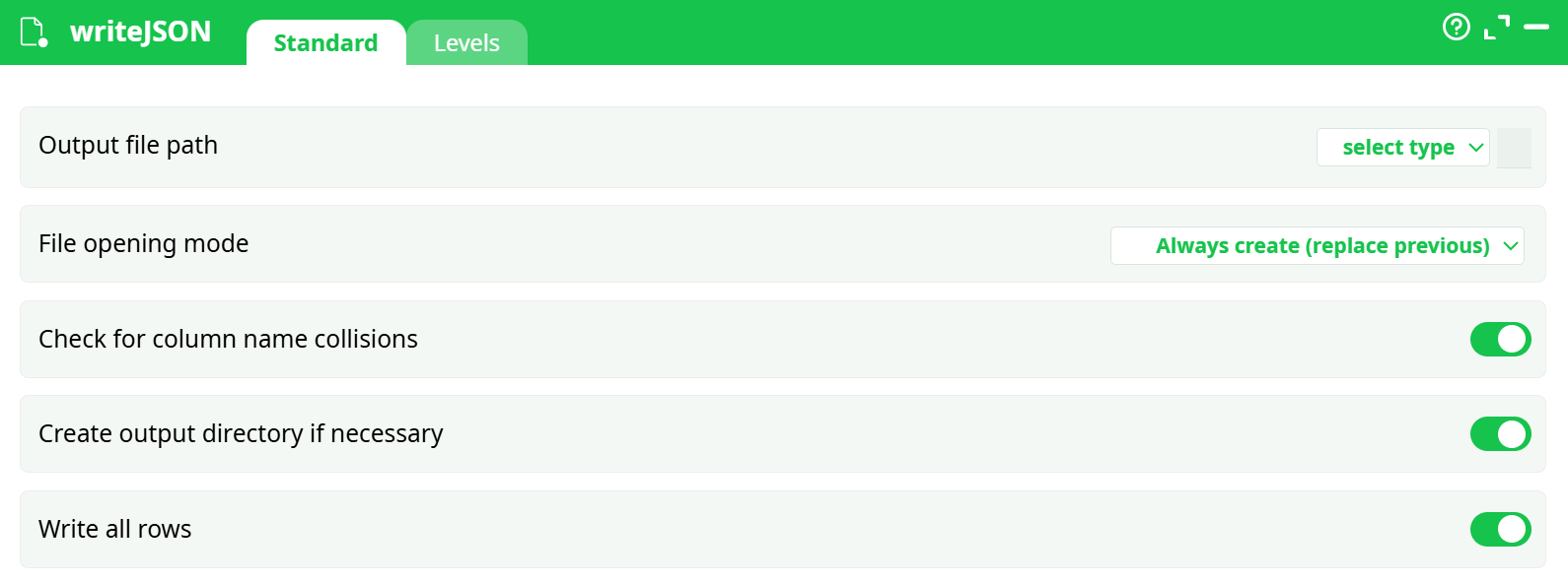
Parameters:
- Output file path
- File opening mode
- Check for column name collisions
- Create output directory if necessary
- Write all rows
¶ Levels Tab
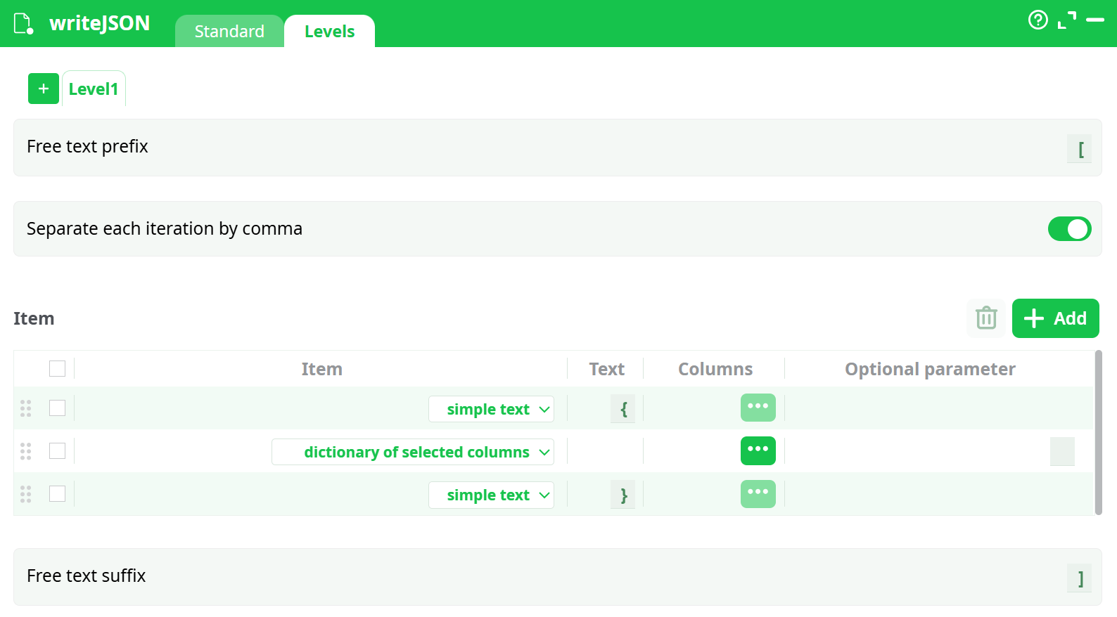
Parameters:
- Free text prefix
- Separate each iteration by comma
- Free text suffix
¶ About
The maximum memory consumption of the writeJSON action is equal to the memory required to store one row of the input table. This means that you can create any JSON file, of any size regardless of the quantity of RAM of your server.
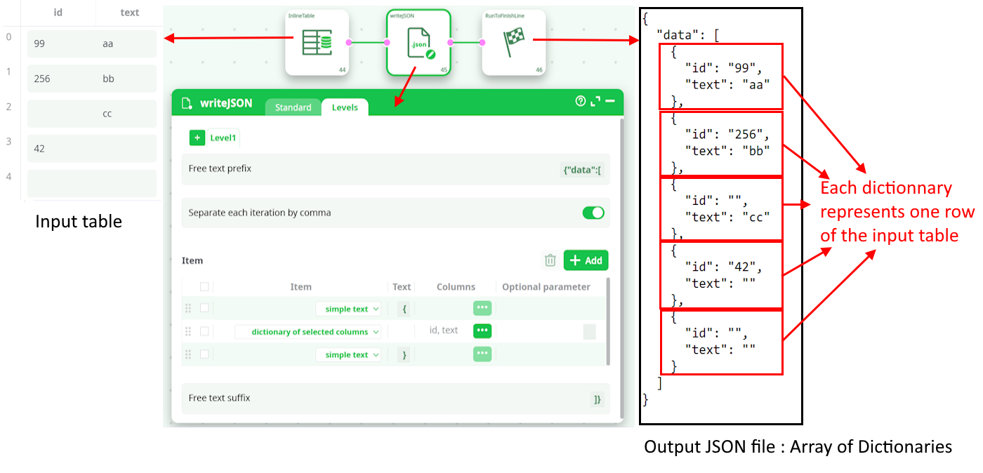
The default settings are producing a simple “one-level” JSON file (you’ll find more information on the “level” principle below) that represents the input table in a quite straight forward way.
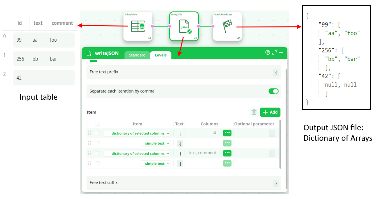
Here are some examples:
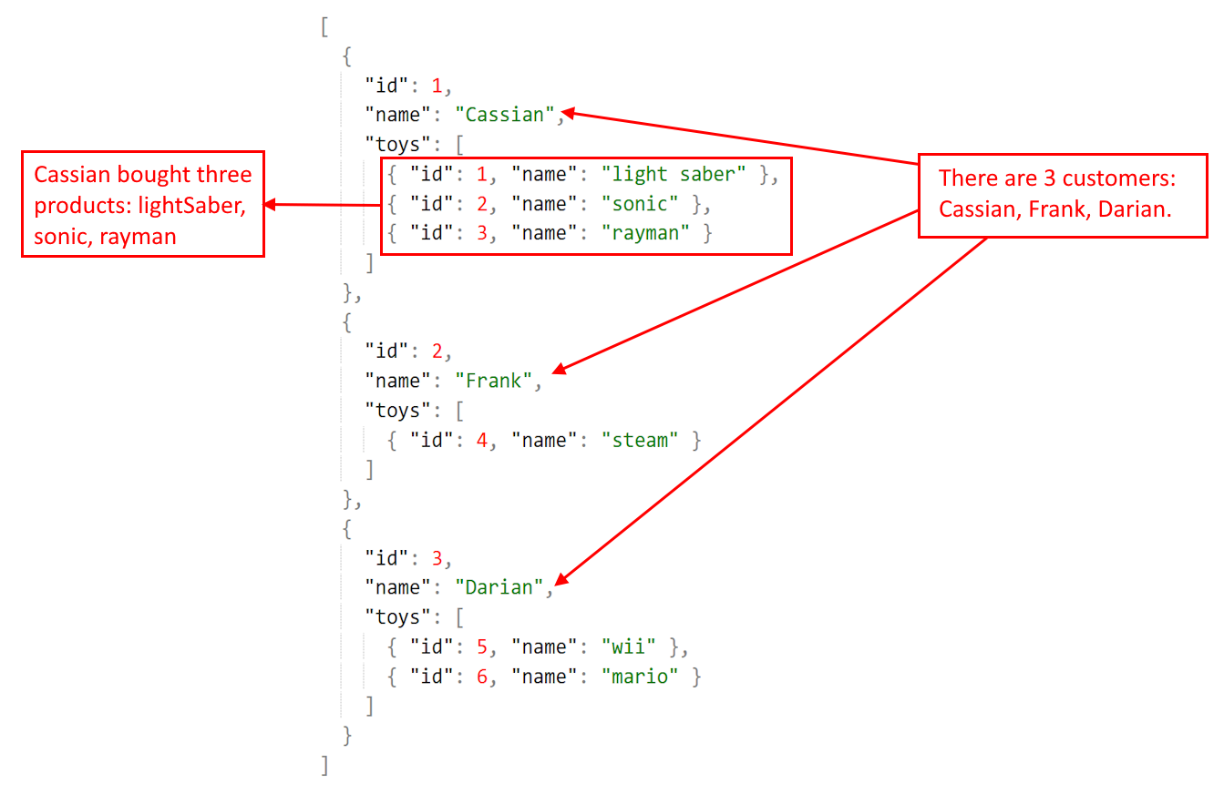
Let’s now assume that you have a JSON file that has a 2-level structure:
• The first, top level contains informations about different customers.
• The second, bottom level contains informations about the purchases of each of the customer.
For example, we’ll have something like this:
The data illustrated in the above JSON file is typically initially stored inside two tables (e.g. a “Customers” table and a “Purchases” table) inside a database. To create the above JSON file, we’ll use the Join action to join these two tables and simply forward the output table inside the writeJSON action : see illustration below:
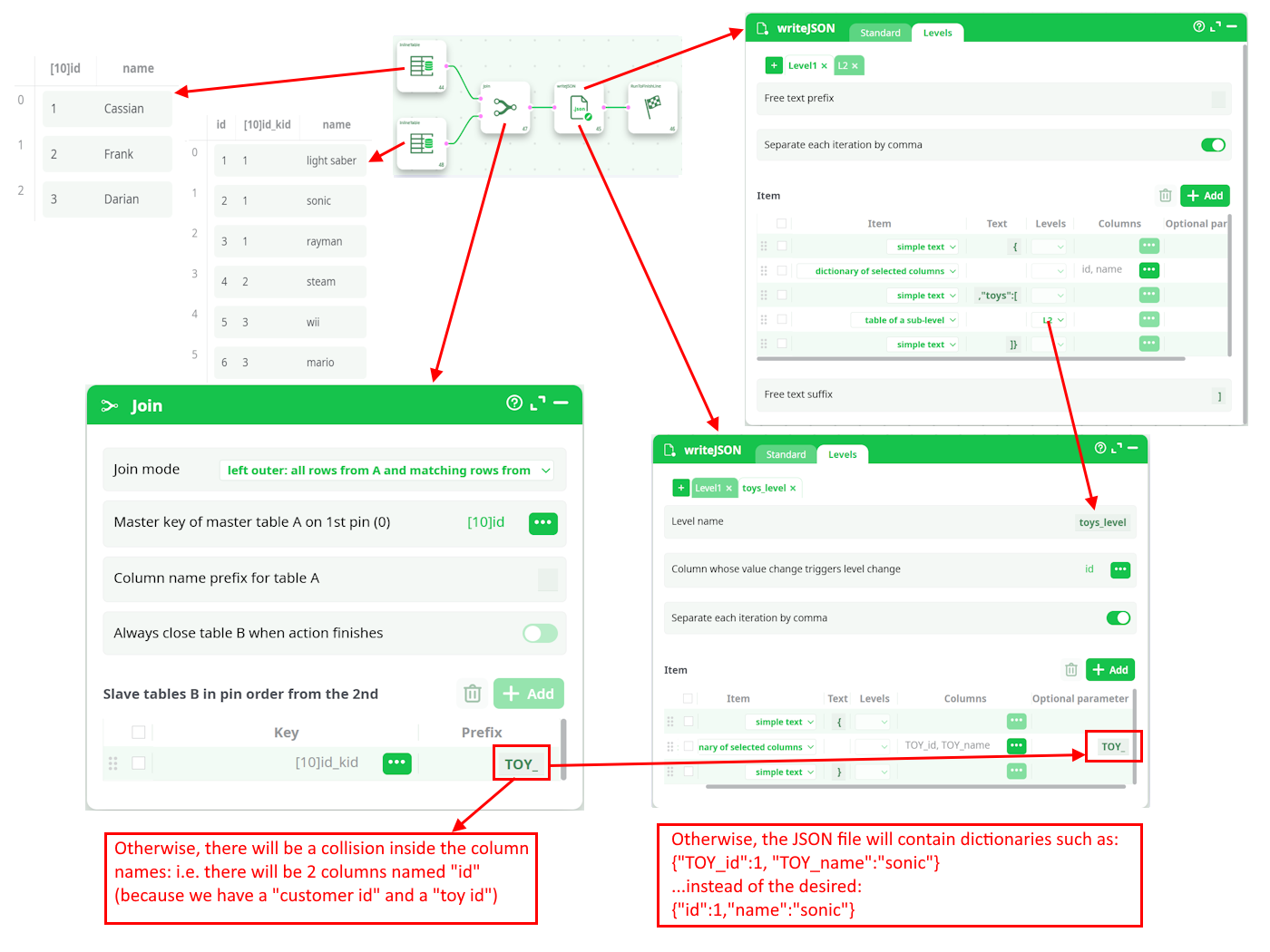
The above example shows you how to create a two-level JSON file (i.e. the levels are “Customers” and “Purchases”). Inside ETL, you can create any JSON files with any number of imbricated levels.
We’ll now introduce a small trick to reduce computation time.
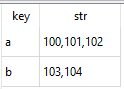
Let’s assume that we want to create the following JSON file:
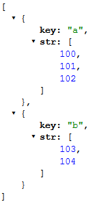
To create the above JSON file, we can use 2 techniques. Here is the first one (that follows the general principles already explained here above):
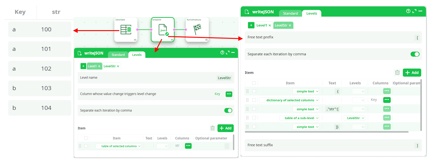
…and here is the second technique:
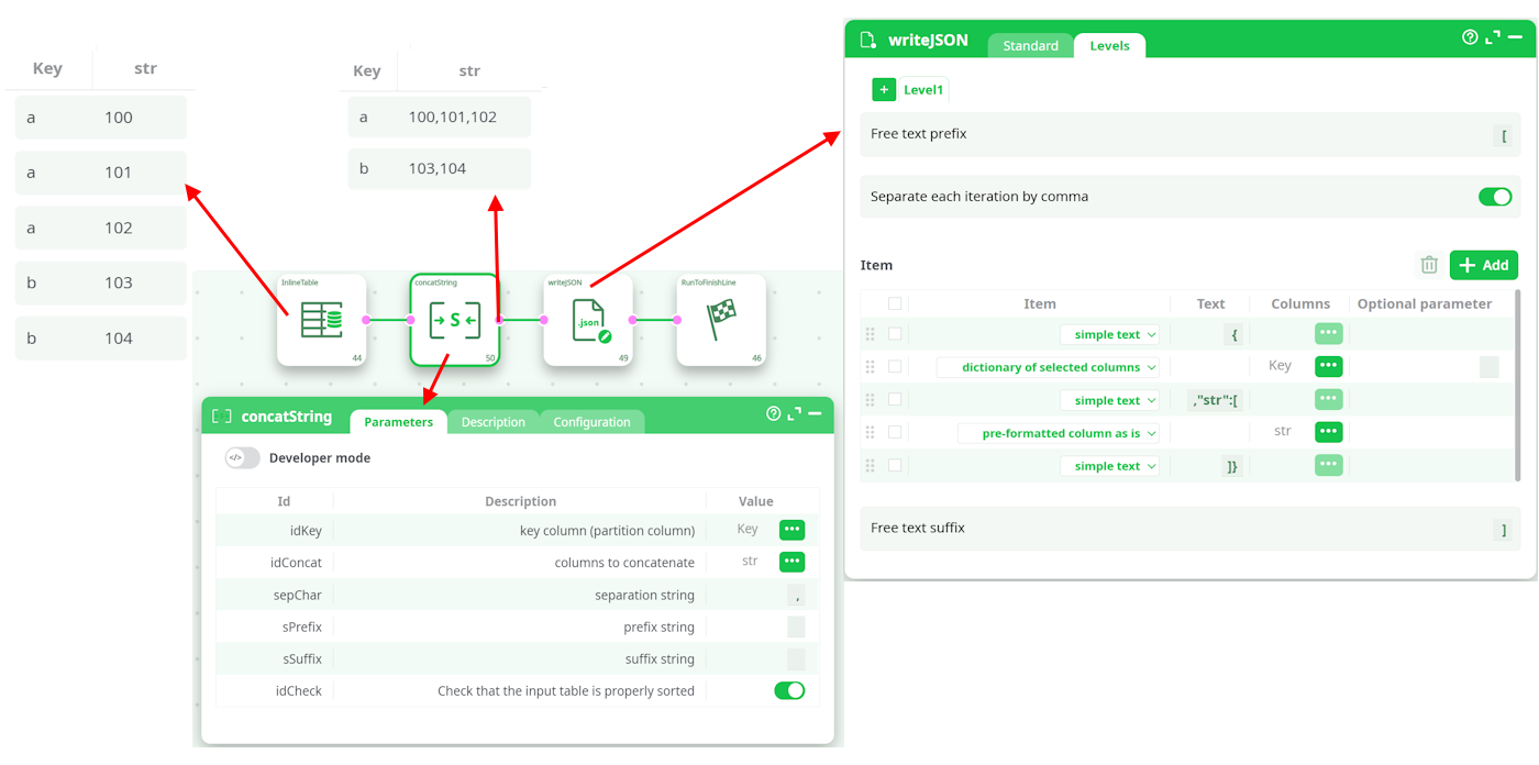
The advantages of the second technique are:
- The input table to the writeJSON action (i.e. the table
 ) has only 2 rows (compared to 5 rows for the first technique). In general, manipulating tables that contain a small quantity of rows leads to a reduced computing time. This is particularly true if the rows are very long (i.e. one thousand columns). The input table in the above example has only a limited number of columns (less than 300), thus the computing-time gain will be inexistent.
 - The input table to the writeJSON action consumes less disk space since there are less un-needed repetitions. For example, you can see that, for the first technique, the key “a” is repeated 3 times while, for the second technique, the key “a” only appears one time.
The disadvantages of the second technique are:
- We were forced to use the concatString: This action is very slow because it involves concatenating a large quantity of (possibly very large) strings (and concatenating many strings is always a slow operation). One trick to lessen the impact of this slow speed is to put the concatString action inside a N-Way multithreaded section.
- The second technique only works for very simple JSON files where we don’t have many different imbricated levels inside the JSON file.
- When using the second technique, we create a row that consumes a large quantity of RAM memory (since the row contains a cell that is the concatenation of all the data required to write the level-2 for a particular level-1). The second technique has thus a quite large memory consumption and it can possibly lead to crashes if the JSON file is too big.