¶ Description
Allows to use several CPU’s/Threads to run the data transformation pipeline.
¶ Parameters
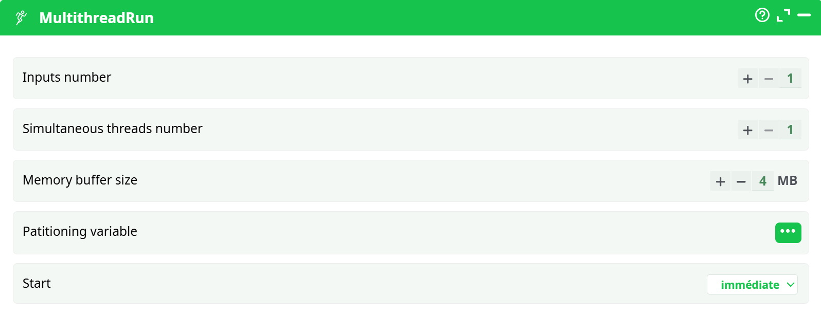
Parameters:
- Inputs number
- Simultaneous thread number
- Memory buffer size
- Partitioning variable
- Start
¶ Defining multithread sections
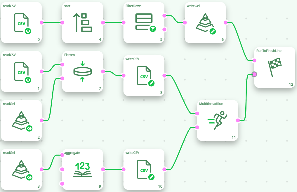
Using the MultithreadRun action, you can cut your data-transformation pipeline in different sections, each section is running on a different CPU. For example, this pipeline runs on 3(+1) CPU’s:
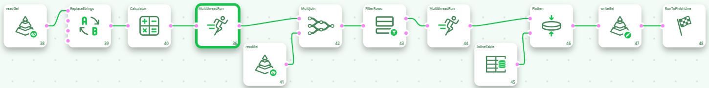
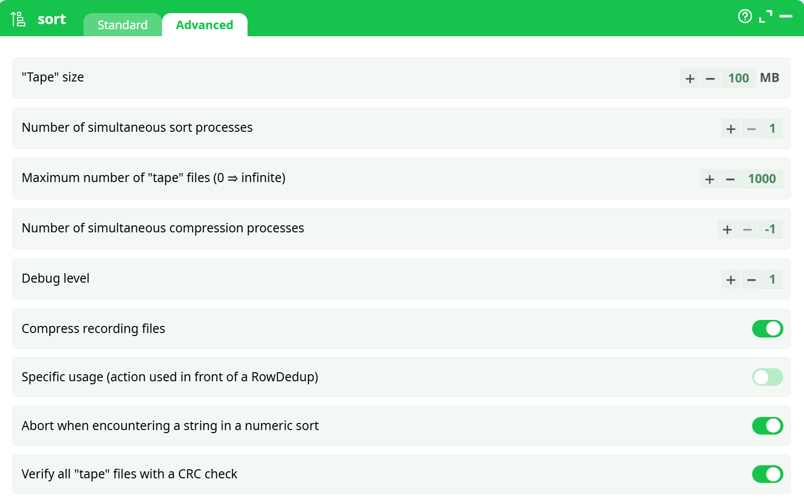
The GelWriter action always use one or more CPU “on its own” to compress the data before writing it on the hard drive. You can change the number of CPU’s used for compression, in the Pipeline Global Parameter window
Inside ETL, the data is processed row-by-row. In the above pipeline, the MultithreadRun action have 2 purposes:
- They are defining the different “Multithreaded Sections”.
- They are passing-by the rows from one section to another. Typically, the different sections are processing the flow of rows at different non-constant speed. To be able to handle the small variations of data flow speed in each section, each Multithread Actions is equipped internally with a FIFO-row-buffer (“FIFO” is a technical terms meaning “First In, First Out”). Schematically, we can represent this FIFO-row-buffer in the following way:
You can think of the FIFO-row-buffer as a water-tank, except that, rather than filling it with water, you fill-it with rows.
If the section on the left of the FIFO-row-buffer is processing the rows at a very high rate (higher than the section on the right), then the FIFO-row-buffer will eventually reach “full capacity”. In such situation, ETL stops the execution of the left section for a little amount of time, so that the FIFO-row-buffer “empties out” a little.
If the section on the right of the FIFO-row-buffer is processing the rows at a very high rate (higher than the section on the left), then the FIFO-row-buffer will eventually be completely emptied out (no rows anymore). In such situation, ETL stops the execution of the right section for a little amount of time, so that the FIFO-row-buffer “fills in” a little. This phenomenon is named “starvation”: The CPU assigned to the right section is “starving” (it does not have enough rows coming in to fulfill its big “appetite”).
To avoid stopping (temporarily) the execution of one of the section of the pipeline, all sections should process the rows at approximately the same speed. If all the sections have more or less the same row-flow-speed the CPU assigned to each section never stops (i.e. there is no “starvation”) and we can reach maximum efficiency: The data-transformation-pipeline is running at maximum speed.
In general, the speed of the data-transformation pipeline is determined by the speed of the slowest multithreaded section (this is the “bottleneck” of the data transformation pipeline).
To avoid starvation (and thus reach maximum processing speed), you must correctly “balance” the workload of each segment.
¶ Balancing Workload in different Multithread Sections
The multiJoin action is usually quite slow (especially when there are many large “slave” tables). Thus, in the example above, the section 2 is the slowest. Section 2 thus drives the processing speed of the whole ETL data-transformation pipeline.
Instead of using 1 CPU to execute the section 2, we could use 4 CPU’s:
A section that is executed using several CPU’s is named a “N-Way” section. To create a “N-Way” section, simply set the parameter “Number of threads” of the Multithread Action to the value 2 or higher.
>NOTE :
You cannot obtain any data preview of the output pins of the Actions included inside a “N-Way” section. To notify you of this limitation, these pins turn RED during pipeline execution. If, for some reason, there exists an HD Cache for a pin that turns RED, it will be deleted.
All HD caches are disabled (and deleted) inside “N-Way” sections. Thus, we suggest you to avoid using “N-Way” sections during the initial ETL pipeline development phase. Once your pipeline has been tested and is working properly, you can start adding “N-Way” sections to increase processing speed.
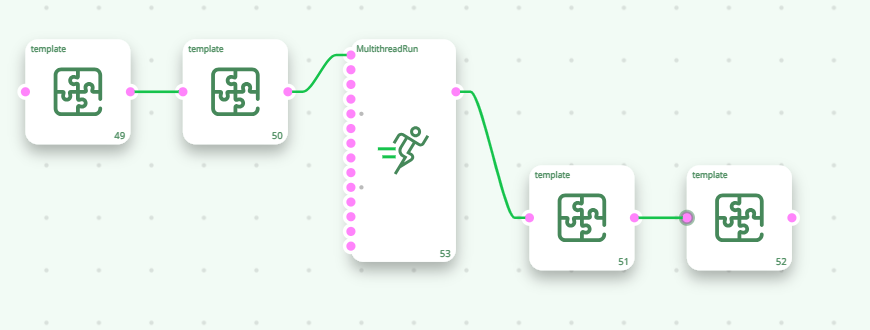
Internally, when you ask to execute a N-Way section, ETL automatically duplicates all the Actions inside the N-Way section and then dispatch a constant “flow of rows” to each of the duplicates. Each duplicate is running “in parallel”, on a different CPU. If we go back to the above example, you could think of the “conceptual” pipeline that is really executed as the following one:
Now, with this new setting (i.e. with 4 CPU’s for section 2), the slowest segment (i.e. the one that drives the global speed of the ETL pipeline) could be section 1 or 3. It can be difficult to adjust properly the number of CPU’s assigned to each section to obtain the highest processing speed. Let’s avoid this difficulty by rewriting the same data transformation in a slightly different way:
The above data transformation pipeline is optimal in terms of execution speed because:
- Section 1 and section 3 are very fast because they each contain only one Action that consumes very little CPU. Thus, if there is a bottleneck, it should be in section 2 (and not in section 1 or 3).
- Section 2 is highly multithreaded (it uses 6 CPU’s). If we could afford more CPU’s, we would use them in section 2 because if, there is a bottleneck, it should be here.
The above pipeline is nearly optimal for a 8-cores CPU (because it exactly uses 8 CPU’s).
However, it can still be improved a little:
- The only Action included in Section 1 is reading a .gel file. Reading a .gel file is a 2 step-process:
- Read a bunch of binary data (typically 1MB) from the Hard Drive and copy into main RAM memory. This takes 90% of the time.
- De-compress the binary data into usable data. This takes 10% of the time.
This means that the CPU assigned to Section 1 will be idle most of the time (90% of the time), simply waiting from the Hard Drive to complete the “Read” (i.e. the “step 1”.). When a CPU is idle, we could use it to execute another section of the pipeline.
- The only Action included in Section 3 is writing a .gel file. Writing a .gel file is a 2 step-process:
- Fill-in an internal memory buffer in RAM with a whole bunch of data (typically 4MB). (5% of the time)
- Tell the compression-thread to compress the data (25% of the time) and flush the data on the hard-drive (i.e. copy the data from main RAM memory to hard drive)(70% of the time).
This means that the CPU assigned to Section 3 will be idle most of the time (70% of the time), simply waiting from the Hard Drive to complete the “Write” (i.e. the “step 2”.). When a CPU is idle, we could use it to execute another section of the pipeline.
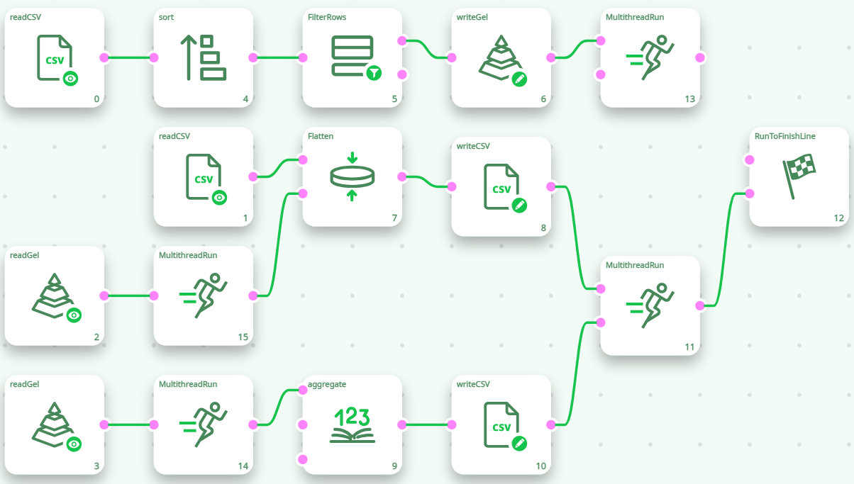
Knowing that the CPU’s assigned to section 1 & 3 will be idle most of the time, we can re-assign these 2 CPU’s to section 2: We finally obtain:
The above pipeline is optimal for a 8-cores CPU (because it exactly uses 8 CPU’s).
¶ Input Actions and Multithread Sections
The readCSV action is “injecting” new rows (that are read from the Hard Drive) into the pipeline. Each time ETL calls the readCSV action, it does the following:
- Look at the internal Row-Buffer of the Action:
- If the Row-buffer is empty:
- Read a bunch of data (typically 1 MB) from the Hard Drive and copy into the Row-Buffer (And, optionally, de-compress the binary data into usable data).
- Select the first row in the buffer.
b. If the Row-Buffer is not empty:
- Select the next row in the buffer
- If the Row-buffer is empty:
- “Inject” the selected row into the ETL pipeline and remove it from the Row-Buffer.
The ReadCSV action is using a synchronous (i.e. blocking) I/O algorithm (See the section 5.2.6.2. about asynchronous I/O algorithms). This means that, while ETL is occupied reading some data from the Hard Drive (when it copies 1MB of data from Hard Drive to main RAM memory), it “freezes” the whole Multithreaded Section that contains the ReadCSV action. To avoid freezing the whole data-transformation-pipeline, it’s a good idea to isolate the ReadCSV Action in a separate Section (thus using a MultithreadRun action).
The same remark applies to all the other “Input Action” that are based on a simple synchronous (i.e. blocking) I/O algorithm: the SASReader action, the [ODBCReader] action, etc. For example, you’ll often have:
You should not use the above combination to increase the running speed of the Action that have asynchronous (i.e. non-blocking) I/O algorithms, these Actions include: the GelReader action, the ColumnarGelFileReader action, the readStat action and the TcpIPReceiveTable action.
Conceptually, the logic is the same with both solution: Use an additional thread to allow the rest of the data-transformation-pipeline to run while the data are extracted from the Hard Drive. The difference comes from FIFO buffer located inside the MultithreadRun action. This FIFO buffer implies a (slow) deep-copy of all the rows that are going through the MultithreadRun action. When using an asynchronous I/O algorithm, you don’t have to perform this deep copy at all and this is thus more efficient.
In this way, when the readCSV action “freezes” (because it’s waiting for the Hard Drive), it only blocks its own Multithreaded-Section but the rest of the transformation pipeline (i.e. the other Sections) can still continue to run (without any interruption), using the rows that are inside the FIFO-row-buffer of the Multithread Action, just next to it. Of course, if it freezes for too long (i.e. if the Hard Drive or the database is very slow), then the the FIFO-row-buffer of the MultithreadRun action empties out and, once again, the whole data-processing stops (this is sometime referred, in technical terms, as a “Pipeline Stall”). This happens very often with the ODBCReader action because the databases systems are usually very slow compared to ETL pipeline: More precisely: Databases have usually some difficulties to “deliver” the rows at the high-speed required by ETL for optimal execution speed. In such common situation, one way to reach high-processing speed is to run “in parallel” different SQL extractions, in different Multithreaded Sections.
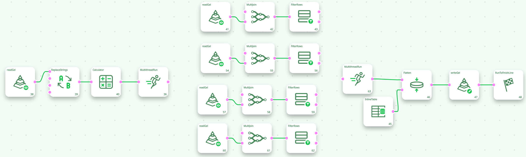
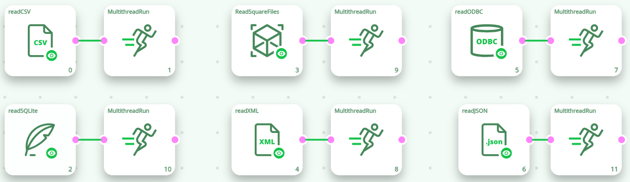
For example, this is not very efficient (despite the fact that it includes several MultithreadRun actions):
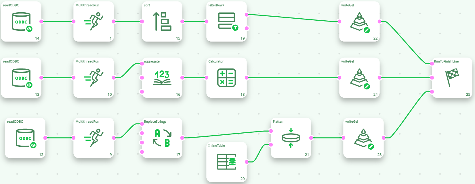
The above pipeline will run the 3 database extractions one after the other and the processing speed will most likely be quite slow because of “Pipeline Stalls”. The following pipline (that runs the 3 database extractions “in parallel”) is a better solution:
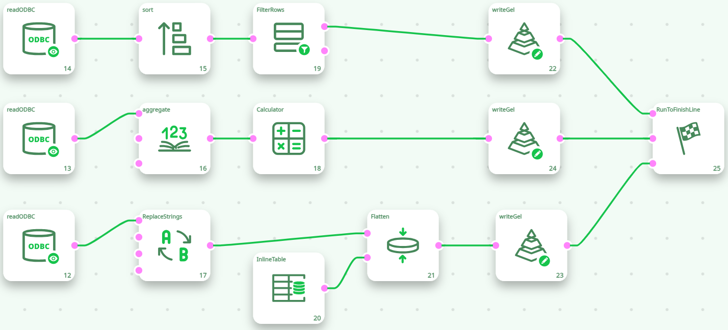
You can think of the MultithreadRun action with several input pins as the “multithreaded” equivalent of the standard RunToFinishLine. The RunToFinishLine executes the pipeline sequentially:
- First, the RunToFinishLine runs all the actions connected to the pin 0.
- Once it’s finished, the RunToFinishLine runs all the actions connected to the pin 1,
- Once it’s finished, the RunToFinishLine runs all the actions connected to the pin 2,
- Once it’s finished, the RunToFinishLine runs all the actions connected to the pin 3, etc.
In opposition, the MultithreadRun action executes the pipeline in parallel. As soon as you run the Pipeline (e.g. as soon as you pressed F5), all the action connected to the MultithreadRun action start running at the same time. You can still have some control on the order in which the actions are executed using the “Synchronization” option of the [MultithreadRun] action.
¶ Limitations of N-Way Multithread Sections
Let’s call “N-Way Sections”, the Multithreaded Sections that are executed using several CPU’s: Such sections are represented using the icon (instead of the “standard” icon). A “N-Way Section” ends with the missing action and always starts with a missing action.
Not all Actions can be included inside N-Way sections. For example, the action or the Join action cannot be included inside a “N-Way Section”. Indeed, if we had the following (non-working) pipeline:

… This would be equivalent to the following “conceptual” pipeline:
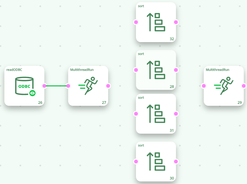
The above illustration explains that each sort action process (i.e. sort) one quarter (¼) of the total number of rows. At this point, we only have a “partial” sort (and not a “complete” sort) because each sort was done on one quarter (¼) of the whole table (and not the whole table). Furthermore, the rows that are “going out” of the sort actions are put together, in a random order, inside the FIFO-Row-Buffer of the “second MultithreadRun action”. Thus, even the (partial) sorting of the row is lost (because of the random order of the rows inside the final FIFO-Row-Buffer on the right).
¶ Overcoming the Limitations of N-Way Multithread Sections
If we have the following ETL pipeline:
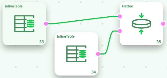
We have a transaction-table, where each row represents one transaction: “How many items of product A or B did the customer X buy?”. Using the “Flatten” Action, we transform this transaction-table into a Customer-table (where each row represents a customer).
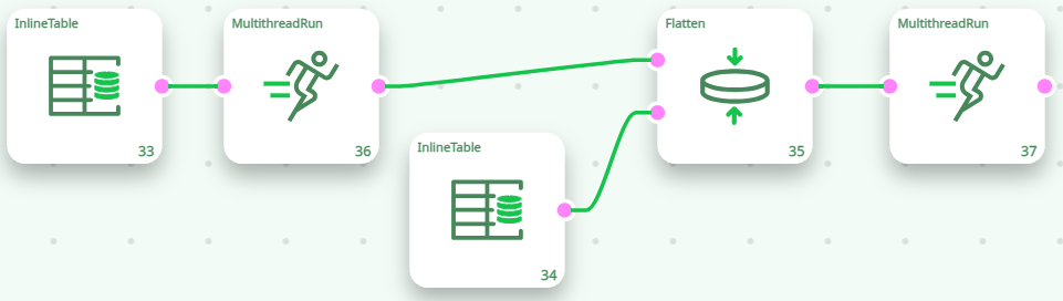
The Flatten action reads the “CustomerID” column in the table on the input pin 0 and, each time the “CustomerID” column changes, it ouputs one row containing all the data about this “CustomerID”. If we execute the Flatten action inside a N-Way Section, we’ll have:
The above pipeline is equivalent to the following “conceptual” pipeline:
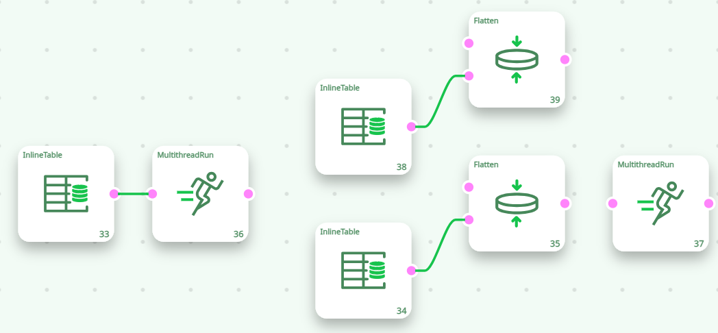
With the default settings, The “Flatten” Action is not working properly inside a N-Way section. We will now see how to correct this situation.
Let’s now define “Branch 1” and “Branch 2”in the following way:
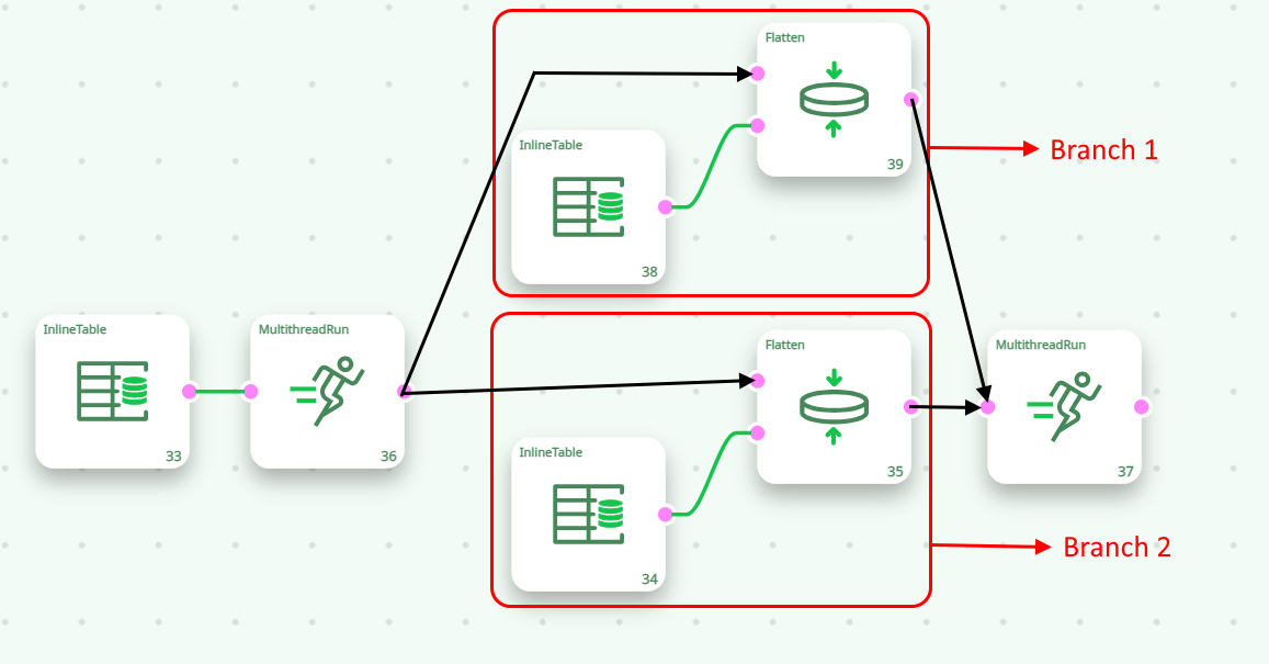
In the above example, the “Flatten” Action inside “Branch 1” receives only a fraction of the rows related to a specific customer (e.g. For the “CostumerID=1”, it receives only the row about the “A” product and nothing about the “B’ product). It thus produced a wrong result (e.g. for the “CostumerID=1”, it outputs only the quantity of A product and nothing for the B product). In order for the The “Flatten” Action inside “Branch 1” to work properly, it should receive all the rows related to a specific customer (e.g. it should receive all the rows related to the “CustomerID=1”). With the default settings, the rows that enter into the first Multithread Action are forwarded more-or-less randomly to either “Branch 1” or “Branch 2”. To guarantee that all the rows related to the same customer are going inside the same branch, we must use the “partitioning” parameter of the Multithread Action: For example, this will work properly:
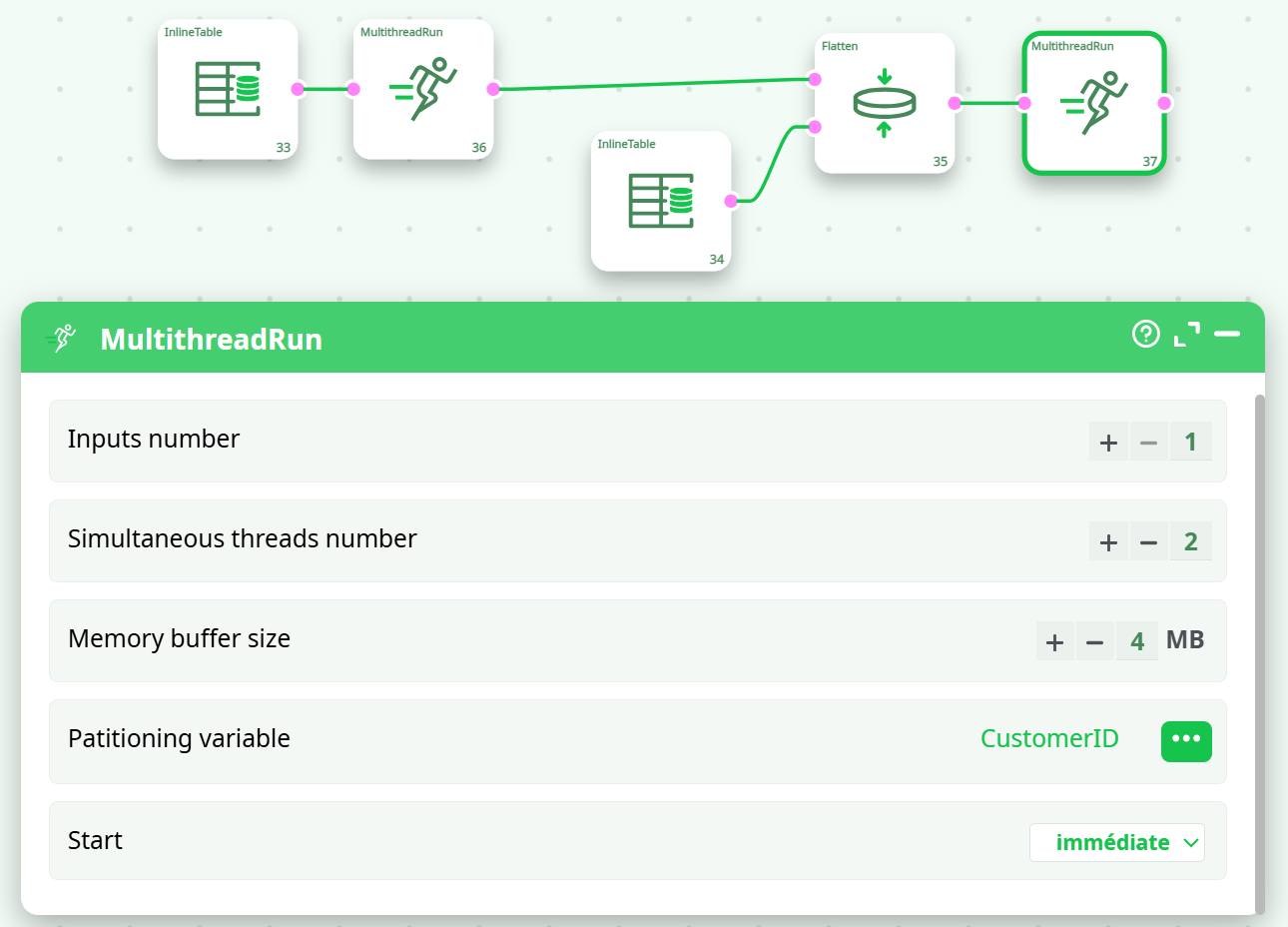
The “partitioning” parameter basically says to the first Multithread Action: “Continue to send the input rows to the same branch, as long as the CostumerID stays the same” (Beware: please note that this “partitioning” parameter is set in the parameter panel of the second Multithread Action). Thanks to the “partitioning” parameter, we can run in parallel an even larger variety of Actions (such as the “Flatten” Action, the Aggregate Action, the Partitioned Sort Action, the kpi_Stock Action, etc.).
To know more about how to overcome the limitations of the N-Way Multithread Section, please refer to section “5.5.5.2. Using the “out-of-memory mode” of the Aggregate Action inside a N-Way Multithreaded Section”.
¶ Thread Synchronization
Let’s now consider the following, erroneous, data-transformation-pipeline:
The above data-transformation-pipeline won’t run properly. Here is why: When we start the execution of the pipeline, the Sections 1, 2 & 3 will all start together, at the same time. In particular, the two ReadGel Actions (that are inside Section 2 and section 3) will directly fail because the file “:/temp.gel” has not been computed yet.
For the above pipeline to run properly, we should wait for complete creation of the “:/temp.gel” file (this is done in Section 1) and, then (and only then), we can start reading the file (in Sections 2 & 3). In other word, we need to wait for the end of the execution of Section 1 before reading the “:/temp.gel” file. This is accomplished in the following way: This will work properly:
Another solution (to ensure that the file “:/temp.gel” is created before any “read” occurs) is the following:
- Copy the section 1 into a file named “section1.age”.
- Copy the sections 2 and 3 into a file named “section2and3.age”.
- Use the runPipelines action to run the two ETL pipelines “section1.age” and “section2and3.age” sequentially (and not in parallel!).
Please note that, although there are three Multithreaded Sections in the above pipeline, it only uses a maximum of 2 CPU’s at the same time (because Section 2 and 3 do not run at the same time as Section 1). This is a common phenomenon. For example:

The above pipeline will NOT use 10+10=20 CPUs. Indeed, Section 2 will run only after the Section 1 is finished (this is because of the sort action that waits until it received all “input” rows before emitting the first “output” row). The above pipeline will thus use a maximum of 12 CPUs.
From the above pipeline, you can see that it’s not possible to run the sort action inside a N-Way section. Does-it mean that all “sorts” are performed using only one CPU? No! The following pipeline computes the 2 “sorts” in parallel and outputs a globally sorted “.gel” file that contains all the data from the 2 input “.gel” files:
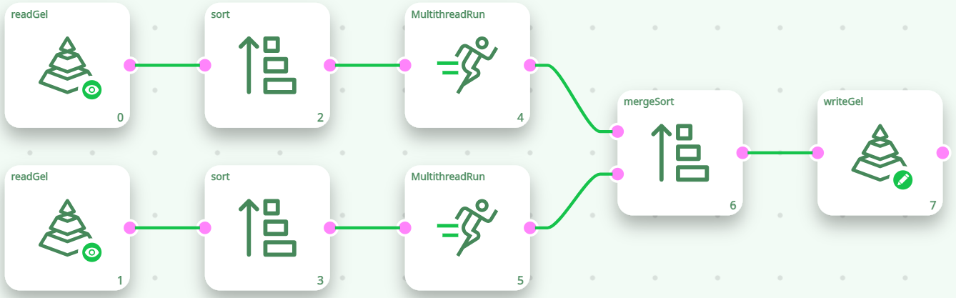
Please note that we used the mergeSort action in order to produce a sorted output (The mergeSort action is the equivalent of the Append action with the slight difference that it produces a sorted output). Using the above technique, it’s possible to use many CPU’s to perform a sort.
¶ Main RAM Memory Consumption
What’s the main RAM memory consumption of the above pipeline?
Each Sort Action consumes 5 GB RAM: Since these two Sort Actions are running in parallel, the total RAM memory consumption of this pipeline is 5GB+5GB=10GB. The same pipeline executed on 1 CPU (i.e. without the Multithread Actions) consumes only 5GB RAM.
When you are executing in parallel some ETL pipeline, the total RAM memory consumption usually increases substantially (compared to the “1-CPU-execution”). In the above example, the memory consumption for the “parallel” execution rises to 10 GB, compared to only 5GB for the simple, “sequential” execution.
If the total RAM memory consumption exceeds the amount of physical RAM inside your computer, then you are in trouble because MSWindows will be forced to “swap” (also named “paging”). When MSWindows “swaps” all processing speed is divided by 100 or more: The computation becomes so slow that it’s better to stop all computation and re-design your data-transformation-pipeline to use less RAM.
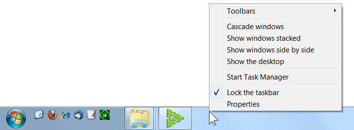
You can check the total physical RAM memory available to you and the memory consumption of your ETL pipelines, by looking at the MSWindows “Task Manager”.
To run the MSWindows “Task Manager”, right-click the MSWindows Taskbar and select “Start Task Manager”:
The amount of total physical RAM memory available to run your pipelines is visible here:
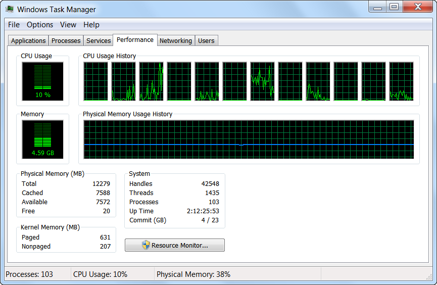
In the above example, I still have 7572 MB ≈ 7.5 GB of Available Physical RAM memory to run my ETL pipelines. When you start your data-transformation-pipeline, ETL start consumming some RAM memory and the amount of Available Physical RAM memory decreases. When this amount drops to zero, MSWindows will start “swapping” and all computations (from the whole computer) nearly stop. You should avoid that!
The Actions that consume a great quantity of RAM memory are:
- The MultiJoin action: This action starts by loading into RAM memory all the Slaves tables (on pin 1 and above). If there are a great quantity of large slave tables, the MultiJoin action will consume a great quantity of RAM.
- The FilterOnKey action: This action works in the same way as the MultiJoin action: It start by leading into RAM memory the table on the second pin. If this table is large, then it will consume a large quantity of RAM.
- The sort action: To sort large table, you need a large “tape size”. It means creating a large buffer into RAM memory (that contains one tape data).
- The aggregate action (when the option “Use in-RAM algorithm for small output tables” is checked): All the output tables (i.e. all the “aggregates”) must fit into RAM memory.
- Most of the action for “Graph Mining” are loading the whole pipeline to analyze into RAM memory. If this pipeline is large, then it will consume a large quantity of RAM. These Actions include the CommunityDetection action, the NodeAnalysis action, the SignificanceLevel action, the Leadership action.
- Most of the Actions for “Operational Research” are loading the whole table to analyze into RAM memory. If this table is large, then it will consume a large quantity of RAM. These Actions include the KNN action and the DatasetReduction action and the AssignmentSolver action.
You should pay extra attention to RAM memory consumption when the above Actions are running in parallel. If you exceed the total amount of Available Physical RAM memory of your computer, all computations will slow down radically.
NOTE :
When using ETL 32-bit (in opposition to ETL 64-bit), the total RAM memory consumption can never >exceed 2 GB. If you try to use more than 2GB RAM, ETL 32-bit will stop (and, most of the time, it will stop >abruptly with the message “segmentation fault”). This limitation is imposed by the hardware and MSWindows.On the contrary, ETL 64-bit does not have any limitation on the total amount of RAM memory that it can use. >However, if you consume more RAM than the total amount of Available Physical RAM memory of your computer, all >computations will slow down dramatically.
NOTE :
Is it possible, using ETL 32-bit, to use more than 2GB RAM memory?
Yes: Using the runPipelines action, you can run several ETL pipelines “in parallel”. Each pipeline runs inside its own process (i.e. inside its own “.exe” application) and uses a maximum of 2GB RAM. The sum of the RAM consumption of different processes can be above 2GB.
¶ Fine-Tuning your script for Best Multithread Speed
You can check if the workload of your different Sections is correctly “balanced”, by looking at the MSWindows “Task Manager”.
To run the MSWindows “Task Manager”, right-click the MSWindows Taskbar and select “Start Task Manager”:
The MSWindows “Task Manager” appears. You can see the number of cores (i.e. this is more or less equivalent to the number of CPU’s) here:
You can see that, on this example, there are 12 cores (i.e. this is more or less equivalent to 12 CPU’s).
You can estimate how much CPU a running ETL pipeline is using. On a 12-core system:
- When ETL fully uses 1 CPU, the “CPU” column displays 8 % (≈1x100/12).
- When ETL fully uses 2 CPU’s, the “CPU” column displays 16 % (≈2x100/12).
- When ETL fully uses 3 CPU’s, the “CPU” column displays 25 % (≈3x100/12).
- When ETL fully uses 4 CPU’s, the “CPU” column displays 33 % (≈4x100/12).
- When ETL fully uses 5 CPU’s, the “CPU” column displays 41 % (≈5x100/12).
If your ETL pipeline is designed to use 4 CPU’s, then the “CPU” column inside the MSWindows “Task Manager” should display 33% (on a computer that has 12 cores). If that’s not the case (e.g. you get 12%), it means that some Multithread Sections are “starving” and you are not completely using your 4 CPU’s. Maybe you should re-design your ETL pipeline to balance in another way the computation workload to better use your 4 CPU’s.
You should also try to avoid using more CPU’s than the than the real physical amount of CPU’s inside your server because, in this situation, MSWindows must “emulate” by software the missing CPU’s and this leads to a very large speed drop: You’ll have “pipeline stall” and “starving” everywhere. For example: you have a 4 CPU server and your ETL pipeline is designed to use 7 CPU’s: This is bad: Your data-transformation will run in very inefficient way: Try decreasing the number of CPU used inside your pipeline.
The “emulation” of many CPU’s involves a procedure named “context switching”: For example, when you emulate two 2 virtual CPU’s using one real CPU’s, what you are actually doing is:
a) Use your (only)real CPU for a few milliseconds to execute the computation that the first virtual CPU must do.
b) Save the “state” of the computation assigned to the first virtual CPU (A “state” typically includes the content of all CPU registers and a reset of the micro-instruction execution pipeline).
c) Restore the “state” of the computation assigned to the second virtual CPU.
d) Use your (only)real CPU for a few milliseconds to execute the computation that the second virtual CPU must do.
e) Save the “state” of the computation assigned to the second virtual CPU.
f) Restore the “state” of the computation assigned to the first virtual CPU.
g) Go back to step a).
The process described in the steps (b) & (c) is one “context switch” (The steps (e) & (f) are also one “context switch”). “Context Switching” consumes a lot of CPU resources. It can happen that 60% of the CPU computational power is used to execute “context switching”. In such situation, only the remaining 40% of the CPU resources are available to compute the data transformation pipeline and it will thus run very slowly.
In the ideal situation, the “Task Manager” should display a number near 100% of CPU-consumption (e.g. 95% or 99%). If you try to use too much CPU’s inside your pipeline (i.e. you try to go “above” 100% of CPU consumption), the computation speed will (most of the time) be reduced. Sometime (not very often), you’ll directly see inside the “Task Manager” that your pipeline is actually slowing down (i.e. the CPU-consumption will drop around 50% because of the many “starvations“). Most of the time, the computational-speed of your data-transformation-pipeline will decrease but it won’t be easily noticeable inside the MSWindows “Task Manager” because you’ll see a 100% CPU-consumption that might fool you (The CPU is actually busy performing many “context switching”).
Adjusting the amount of CPU used inside a pipeline can be tricky: We are always tempted to design our pipelines to use more and more CPU’s. But, at the same time, if we try to go “above” 100% of CPU consumption, the data-transformation suddenly slows down dramatically. Finding the right settings sometime requires a small “trial-and-error” procedure to get it right. Simply “time” your transformation pipeline on a sample, using different settings and keep the settings with the shortest computation time.
Be warned: There is a BIG penalty-hit if you try to use more CPU’s than actually physically available inside your server. In the ideal situation, the “Task Manager” should display a number near 100% of CPU-consumption (i.e. 95% or 99%).
NOTE :
Why is it so bad to try to use more CPU’s than the actual number of physically available CPU’s inside your server?One first, simple answer is that you’ll lose CPU resources in “context switching”. …but there is something even worse than that.
Let’s assume that you have a 2-CPU server and you run this pipeline:
This pipeline is designed to use (at least) 5 CPU’s. In between each of the 5 multithread segments, there is a Multithread Action that contains a FIFO-Row-Buffer (do you remember the “water tank” of section 5.3.2.1.?).Let’s now assume that SEGMENT 5 is very fast to compute. Thus, most of the time, the FIFO-ROW-BUFFER 4 will be empty (because, as soon, as there are a few rows inside the buffer, we’ll process them all very quickly). In technical terms, SEGMENT 5 is “starving” most of the time. To give some rows to process to SEGMENT 5, we need to run SEGMENT 4 for a little while. …but we have only 2 real CPU’s: The MSWindow task scheduler must assign one of the 2 real CPU’s to SEGMENT 4. The MSWindow scheduler has no idea of the structure of your data-transformation-pipeline: It does not know about the dependencies that exist between the different SEGMENTS: e.g. It has no idea that, to un-block SEGMENT 5, it needs to run the SEGMENT 4 for a little while. Thus, it will choose mostly randomly one of the SEGMENTS to run. If you are lucky, it will be SEGMENT 4 and your data-transformation will “advance” a little bit further. If you are unlucky, it will choose a SEGMENT that has an input FIFO-ROW-BUFFER nearly empty: This SEGMENT will thus run for a very small amount of time (to process the small number of rows in input) and then stop (i.e. because of “starvation”: no more rows to process), forcing the MSWindow task scheduler to execute one more CPU-costly “context switch” (searching for another SEGMENT to run). This will lead to a large amount of “context switching” (searching for the “right” multithread segments to SEGMENT to “advance” the data transformation) and, at the end, you obtain a very inefficient (i.e. really slow) data transformation.
Some poorly designed Multi-CPU multithreaded ETL pipelines might run slower than their 1-CPU single threaded equivalent (it’s quite common for very small pipelines, with only a few Actions). It’s also common that some ETL pipelines should not be multithreaded at all (More precisely: Any pipeline can be multithreaded: The question is rather: Does the multithreading makes computation faster?).
Summary: Because the MSWindow task scheduler does not know about the dependencies between the different multithread SEGMENTS inside your data transformation pipelines, it will lose a large amount of CPU-time in “context switching”, searching (mostly randomly) for the “right” SEGMENT to execute. This, of course, leads to very slow computing speed for your data transformation. Do not design your pipeline to use more CPU’s than required. Sometime, 1-CPU single-threaded execution is the fastest.

¶ About multithreading inside other ETL’s
Most ETL’s do not have multithreading functionalities. Some are using a very specific (and primitive) form of multithreading: They automatically insert a MultithreadRun action in-between every normal action. For example, when you see the following data-transformation pipeline inside a “classical multithreaded ETL tool”:
… this is, in reality, executed in the following way (note that we simply inserted a Multithread Action in-between every Action):

This means that, if you have a pipeline with twenty Actions, there will be (roughly) twenty CPU’s used to run the data-transformation-pipeline. Twenty is a number that is (usually) significantly larger than the physical amount of available CPU’s and this pipeline will thus run very slowly (because of the software “emulation” of the missing CPU’s performed by MSWindows: See the previous section about this subject). There is no way of preventing that.
Each MultithreadRun action has an internal FIFO-row-buffer. The management of this FIFO-row-buffer consumes a big amount of precious CPU time. Thus, it’s a good idea to reduce to the minimum the number of Multithread actions in your pipeline: you can do that by designing your pipeline so that it has the longest Sections as possible (i.e. a section should include as many actions as possible).
The data-transformation-engines that are used inside “classical” multithread ETL’s are using a very large amount of FIFO-row-buffers (because they internally place a MultithreadRun action in-between every action: All their sections are composed of only ONE action it’s terrible!) and they are thus losing a very large amount of precious CPU time in managing all these un-necessary FIFO-row-buffers (and also in “context switching”).
Most “classical” multithread ETL Engines do not even offer the equivalent of “N-Way Multithreaded Sections”.
In opposition, inside ETL, you have the complete control of:
a) how many CPU’s your data-transformation is using.
b) how many FIFO-row-buffers your data-transformation is using.
This “total control” allows you to use in the most efficient way, all the CPU’s inside your server.
¶ Summary
The [MultithreadRun] action has 3 operating modes:
- This defines the border between 2 simple Multithread Sections. Simple Multithread Sections do not alter the order (i.e. the sorting) of the rows. It means that you can safely put these a little bit everywhere in the data transformation pipeline.
- This defines a N-Way Multithread Section (that is located just BEFORE the Multithread Action and NOT AFTER). The rows that exit a N-Way Multithread Section are not sorted anymore (i.e. N-Way Multithread Sections are removing all “sorting attributes” in the flow). You can use a partitioning variable to better control which rows are sent to which branch/CPU. Inside a N-Way Multithread Section you cannot have any HD cache.
- This is the multithreaded equivalent of the GlobalRunFlag Action. All the actions connected to the input pins of the Action are starting & running simultaneously.
Always design your data-transformation-pipeline without any multithreading. Once everything has been tested and is working properly, you can start adding Multithread Actions to improve processing speed.
You should try to use the minimum amount of MultithreadRun actions because the management of the FIFO-row-buffer (that is included inside the MultithreadRun action) consumes precious CPU time (The MultithreadRun actions are a special case because they do not have any internal FIFO-row-buffer, because they output nothing, so you can have plenty of them). In the same spirit, always try to make the longest Sections as possible. A Section should include as many actions as possible.
Combining together an Input-Action with a MultithreadRun action is usually a good idea (but not for the GelReader action, the ColumnarGelFileReader action, the readStat action and the TcpIPReceiveTable action).
Use the MSWindows “Task Manager” to:
a) Optimize your multithread parameters (i.e. the position and the content of the different Sections and the number of CPU assigned to each Section): Do not try to use more than 100% of CPU consumption: it will directly translate to a large efficiency penalty.
b) Optimize the memory consumption of your pipeline.
- When using ETL 64-bit, do not use more RAM memory than the physical memory available inside your computer.
- When using ETL 32-bit, do not use more than 2GB RAM memory.